Differential Operators, Surface Signals, and the Hidden Mathematics of Mesh Editing

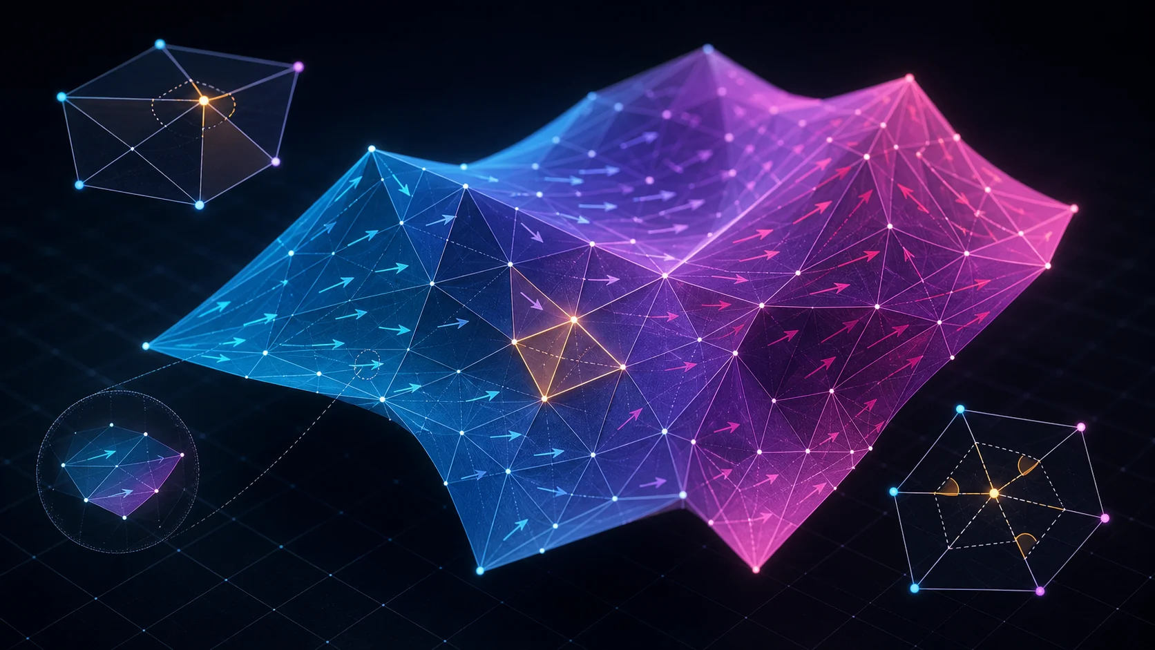
In the previous chapter, we built a broad map of geometry processing. We looked at meshes, simplification, parameterization, deformation, painting, reconstruction, and the internal logic behind tools such as Maya, Houdini, Nuke, and sculpting applications. Now we go deeper into the machinery underneath those techniques.

Once we think of attributes as signals, geometry processing starts to resemble signal processing. An image is a signal defined on a rectangular grid. Audio is a signal defined over time. A mesh attribute is a signal defined over an irregular curved domain.

The challenge is that a mesh does not have the regular structure of an image. Vertices are unevenly spaced. Triangles vary in size and orientation. Connectivity is irregular, and the surface curves through space. Yet we still want to blur, sharpen, differentiate, interpolate, compress, segment, filter, and analyse its signals. This requires discrete differential operators.

Part OneA Surface as a Computational Domain

Imagine a digital terrain. At each point, we might store elevation, moisture, vegetation density, erosion rate, or snow depth. The terrain itself is geometry; all of those additional quantities are fields defined over it.

Now imagine a character. Every surface point may carry skinning weights, material assignments, subsurface-scattering parameters, blood-flow values, wrinkle intensity, cloth-contact pressure, and local deformation strain. Many artists see visible polygons. Many algorithms see a network that supports functions.

A function on a mesh assigns a value to every vertex, face, edge, or surface point. A scalar function assigns one number. A vector function assigns direction and magnitude. A tensor field can encode structured directional behaviour such as anisotropic stiffness or stretch.

Once a field exists, we can ask how it changes. Does it vary quickly or slowly? Where are its maxima? In which direction does it flow? Can we reconstruct it from sparse samples? Those questions lead to gradient, divergence, curl, and Laplacian operators.

Part TwoThe Gradient on a Surface

The gradient points in the direction in which a scalar quantity increases most rapidly. On a grayscale image ramp, it points toward increasing brightness, and its magnitude says how quickly brightness changes.

On a surface, the same intuition applies, except that the gradient must lie tangent to the surface. If one side of a metal statue is hot and the other cold, the gradient points along the statue toward the fastest temperature increase. It does not point into empty space.

This makes the surface gradient intrinsic: it describes change experienced by something moving along the mesh. For a distance field, the negative gradient points approximately along the shortest route back to the source. For a UV coordinate, its gradient describes local parameter direction and texture density. For a painted height field, it points up the steepest surface ascent.

Part ThreePiecewise Linear Fields on Triangle Meshes

A common mesh function stores one value at every vertex and linearly interpolates those values inside each triangle. The field is continuous, but its rate of change may jump across triangle boundaries.

Within one flat triangle, the gradient is constant. A linearly interpolated scalar field forms a tilted plane in value space; the direction and steepness of that tilt are the gradient. This gives us a beautifully practical strategy: compute local differential quantities per triangle, then assemble them into a global operator.

Piecewise-linear finite elements are simple enough to evaluate efficiently and expressive enough to approximate smooth differential behaviour as a reasonable triangulation is refined.

Part FourDivergence

Divergence measures how much a vector field behaves like a source or a sink. If arrows spread outward from a point, divergence is positive. If they converge, it is negative. If flow passes through without accumulating or dispersing, it is near zero.

On a surface, those arrows live in tangent planes. In fluid simulation, divergence tells us whether a velocity field expands or compresses material; incompressible flow aims for zero divergence. In geometry processing, divergence also helps convert a vector field back into a scalar field.

If we know the desired gradient of a height function, taking its divergence and solving a related equation lets us reconstruct the height. That pattern appears in Poisson image editing, normal integration, surface reconstruction, gradient-domain mesh processing, and parameterization.

Part FiveThe Laplacian

The Laplacian is the central operator in geometry processing. Intuitively, it measures how a value differs from its neighbourhood. A vertex far above its local average is a peak; one far below is a valley. A field varying linearly through the neighbourhood has a Laplacian near zero.

The operator can act on temperature, colour, displacement, vertex coordinates, or any compatible signal. On temperature it drives diffusion. On colour it smooths. On position it relates to curvature. In an optimization it spreads constraints. When diagonalized, it reveals the natural frequencies of the shape.

Part SixWhy Averaging Is Not Enough

A naive “umbrella” Laplacian subtracts the average of neighbouring vertex values from the current value. It is easy to implement, but ignores geometry: a nearby vertex and a distant vertex receive equal weight, and a tiny triangle may influence the result as much as a large one.

Principled Laplacians use weights based on local triangle geometry. The most famous is the cotangent Laplacian. Its edge weights depend on the angles opposite an edge, arise naturally from finite-element reasoning, and connect to Dirichlet energy.

On well-shaped meshes it performs exceptionally well. On extreme or inverted triangles it can behave less intuitively. This exposes an important production truth: poor triangles do not merely look untidy; they alter the numerical behaviour of the tools operating on them.

Part SevenCotangent Weights, Intuitively

For two vertices connected by an edge, the surrounding angles describe how strongly the surface supports variation across that connection. Broad, well-supported geometry contributes differently from a narrow, skinny configuration.

The resulting operator is symmetric, respects local geometry, and arises from minimizing variation over the surface. Under suitable mesh conditions, it converges toward the smooth Laplace–Beltrami operator as triangles are refined.

Laplace–Beltrami is the surface-aware Laplacian. It is intrinsic: it depends on distances and angles measured within the surface, not merely on where the surface sits in world space. Bend a sheet without stretching it and its intrinsic differential structure remains essentially the same.

Part EightMass Matrices and Area

Vertices do not all represent equal surface area. One may be surrounded by broad triangles while another sits inside a dense patch. If they are treated equally, integrals, diffusion, spectral analysis, and curvature estimates become biased.

A mass matrix assigns an effective area to every basis function or vertex. It translates discrete sums into approximations of continuous surface integrals. Barycentric area divides each triangle equally. Voronoi-like areas allocate regions by geometric proximity, while mixed areas handle obtuse triangles carefully.

The mass matrix looks like bookkeeping, but it establishes what each degree of freedom represents. In generalized spectral problems, the stiffness matrix says how much a signal varies and the mass matrix says how much surface carries that variation.

Part NineThe Laplacian of Position and Mean Curvature

Apply the surface Laplacian to the mesh’s own 3D position coordinates. The result points approximately in the normal direction and is related to mean curvature. On a flat patch it is near zero. On a curved region it points toward the direction in which the surface moves under mean-curvature flow.

This explains why ordinary Laplacian smoothing shrinks geometry. Small bumps disappear, thin features contract, and closed convex surfaces become rounder and smaller. The mathematics is elegant, but artistically dangerous because intentional detail and scanning noise are both high-frequency signals.

Part TenExplicit and Implicit Smoothing

Explicit smoothing computes the current Laplacian, moves vertices a small distance, and repeats. It is intuitive and cheap per step, but large time steps become unstable; a mesh can oscillate or explode.

Implicit smoothing defines the new state through an equation that includes the new state itself. It requires solving a sparse linear system but remains stable for much larger steps. That trade—more work per step for far better stability—appears throughout geometry and simulation.

Stability is not the same as fidelity. An implicit solver can stably converge to a badly shrunken surface. Time integration controls numerical behaviour; the energy and constraints control what “better” geometry means.

Part ElevenTaubin Smoothing

Taubin smoothing alternates a smoothing step with a smaller reverse-smoothing step. The first removes high-frequency variation; the second expands slightly. With carefully chosen strengths, noise is suppressed while overall scale is less affected.

Conceptually it behaves like a mesh filter with a designed frequency response. It was an early, practical example of spectral thinking: stop calling smoothing “averaging” and ask exactly which frequencies should be attenuated.

Part TwelveBilateral Mesh Filtering

An image bilateral filter considers both spatial proximity and value similarity. Nearby pixels influence one another strongly only when their colours or intensities are also similar.

On a surface, we can compare positions and normals. Nearby faces with similar normals probably belong to the same smooth region. Faces with very different normals may sit across a designed crease, so their influence should be reduced.

This reveals a general feature-preservation principle: define more than one notion of distance. Two samples may be close in space but far apart in orientation, material, visibility, or semantics.

Part ThirteenNormal Filtering

Many denoisers smooth the normal field before moving vertices. This separates orientation from location. A scanned plane may have noisy positions and wobbling triangle normals. Smooth those normals toward a coherent direction, then reconstruct positions consistent with them, and the plane becomes clean.

Sharp edges can survive when averaging stops across large angular differences. The workflow is two-stage: infer a desirable orientation field, then solve for geometry matching it. This resembles gradient-domain image processing and often preserves structure better than direct coordinate smoothing.

Part FourteenGradient-Domain Processing

Poisson image editing changes gradients instead of pixels. It can preserve texture while replacing broad lighting, or insert one object’s edge structure into another image and reconstruct consistent colours.

Meshes support the same philosophy. We manipulate edge vectors, face gradients, local differential coordinates, or normals, then reconstruct global vertex positions. Local detail lives naturally in derivatives: a wrinkle is not primarily an absolute position but a pattern of changing directions and offsets.

That is why differential coordinates are valuable in deformation. Large-scale control motion can change the global pose while a reconstruction energy carries the local surface language along with it.

Part FifteenPoisson Reconstruction Intuition

Suppose a vector field is intended to be the gradient of an unknown scalar function. Measurements are noisy, so no exact scalar function matches every vector. A Poisson solve finds the function whose gradient best matches the field overall in a least-squares sense.

Think of reconstructing terrain from slopes. If someone gives you the desired uphill direction everywhere, the solver builds the most consistent height field. The unknown may instead be surface coordinates, deformation coordinates, depth, texture values, or an implicit occupancy field.

Poisson systems recur because derivatives are often easier to measure, transfer, or edit than absolute values—and because a global solve can reconcile millions of imperfect local suggestions.

Part SixteenHarmonic Functions

A harmonic function has zero Laplacian in the interior. Every unconstrained value equals a weighted average of its neighbours. There are no interior peaks or pits unless boundary conditions force them.

This is the equilibrium of heat with fixed boundary temperatures. Hold the left edge of a metal plate cold and the right edge hot; after enough time the temperature becomes harmonic, smoothly interpolating between them.

Harmonic functions are used for parameterization, selection falloff, interpolation, weights, deformation, and coordinate construction. They are smooth and stable, but not magically rigid or volume preserving. They propagate influence; the designer must still decide what that influence means.

Part SeventeenHarmonic Coordinates for Deformation

Enclose a character in a cage and assign every interior point weights relative to cage vertices. For one cage vertex, fix its weight to one there and zero at the other controls; let the value vary harmonically throughout the volume. Repeat for every cage vertex.

The weights sum to one and reconstruct an interior point as a weighted combination of cage positions. Unlike direct distance weights, harmonic influence travels through the domain, respecting shape and obstacles. This produces smooth, shape-aware deformation, though volumetric solves can be expensive.

Part EighteenBiharmonic Functions

Harmonic interpolation minimizes first-order variation. Biharmonic interpolation uses a higher-order smoothness objective, producing gradients that themselves change smoothly and influence regions that feel broad and natural.

Bounded biharmonic weights are popular for skinning and cage deformation because they satisfy control constraints without the abrupt transitions of simpler schemes. “Biharmonic” sounds abstract, but its intuition is direct: harmonic methods avoid unnecessary slope; biharmonic methods also avoid unnecessary changes in slope.

Closing PerspectiveWhat This Changes in Practice

When a mesh tool behaves strangely, ask three questions. What field is being processed? Which discrete operator is being used? What geometry and area weighting define the operator?

A smoothing slider may hide an explicit time step, an implicit solve, a bilateral normal filter, or a spectral transfer function. A deformation tool may interpolate positions, preserve differential coordinates, or solve a biharmonic energy. A “curvature” mask may be an umbrella estimate or a mass-normalized cotangent operator.

Understanding that hidden machinery changes how you diagnose artifacts. It explains why remeshing improves some operations, why UV and colour signals need explicit preservation, why skinny triangles poison otherwise sound mathematics, and why a stable solver can still produce the wrong artistic result.